---
title: "Is $10,000 Enough? Industrial Land Proximity, Income Gradients, and the Cost of Living Next to a Facility"
author: "Raul Sola Navarro"
date: "2026-10-04"
date-modified: "2026-10-07"
format:
html:
toc: true
toc-depth: 3
code-fold: true
code-tools: true
theme: cosmo
fig-width: 10
fig-height: 8
execute:
echo: true
warning: false
message: false
---
## Introduction
In June 2026, NorthPoint Development offered 4,500 households in Hazle
Township, Pennsylvania $10,000 each -- in cash -- if they would support
approval of a 1,300-acre data center in their community. Locals pushed back,
calling it a bribe. The township had already rejected the project on zoning
grounds and enacted a moratorium on data center construction. The median
household income in the area is around $60,000.
That offer crystallizes a question that is now live in communities across the
United States: **when a large industrial facility is proposed near a residential
area, how much should affected residents actually be compensated -- and how
would you even calculate the right number?**
The AI data center buildout has made this question urgent. In Q2 2026 alone,
community resistance blocked or delayed 45 data center projects worth $68
billion across the U.S., according to [Data Center Watch via
parameter.io](https://parameter.io/community-resistance-stalls-68-billion-worth-of-ai-data-center-developments/).
The [Brookings Institution](https://www.brookings.edu/articles/data-center-backlash-signals-a-fight-over-ai-power/)
framed the backlash as a proxy for a broader question: who decides where AI
infrastructure goes, and who bears its costs?
Residents object for concrete reasons -- noise, water use, power consumption,
and the suspicion that nearby homes will lose value. That last concern is
empirically grounded. A [2011 hedonic pricing study from the
Netherlands](https://papers.tinbergen.nl/09035.pdf) (de Vor & de Groot, using
data on 70,684 home sales) found that homes within 250 meters of industrial
sites sold for roughly 15% less than comparable homes beyond 2,250 meters --
a discount that fades to near zero by about 1.4 miles out. Research
specifically on data centers is more mixed. A [November 2025 George Mason University study](https://schar.gmu.edu/news/2025-11/study-home-prices-are-higher-when-house-near-data-center)
on Northern Virginia home sales found prices *higher* near data centers -- but
Northern Virginia is an atypical case: a high-income tech corridor where the
data center industry is already integrated into the local economy and a major
employer. Resident complaints near operating facilities (noise from cooling
equipment, power infrastructure, and truck deliveries) are documented in local
press from Georgia, Ohio, and Virginia, but rigorous before-and-after property
value studies at specific data center sites are not yet publicly available.
None of this research answers the compensation question directly, because it
describes outcomes -- what actually happened to property values in places that
already have industrial land -- not what should happen in places considering
it. To get at that, you need to know what living near industrial land
correlates with in terms of income and revealed preference, across many
communities and many distance bands.
**That is what this analysis provides, for New York City.**
---
### What This Project Started As
This report began as a logistics gap analysis. The original question was
narrow: which NYC census tracts fall outside a 1-mile radius of any industrial
lot, and how many residents live in those gaps? The spatial analysis answered
that -- 31 tracts, 61,426 residents, concentrated in outer Queens and Brooklyn.
When I added income data, the logistics framing became secondary. **Median
household income rises monotonically with distance from industrial land across
every distance band.** The income gap between tracts within 0.5 miles of
industrial land and those beyond 0.5 miles is roughly $18,000 at the median
-- a pattern that is statistically robust but reflects sorting, not a
directly measurable cost.
That finding connects to the NorthPoint / Hazle Township situation via the
Netherlands property value research. If a home near the proposed facility
is worth $200,000 and industrial proximity discounts it by 15%, that is a
$30,000 loss in asset value -- three times the NorthPoint offer. The NYC
income gradient points in the same direction but is a sorting signal, not a
cost figure. The Dutch property value evidence is the more direct benchmark,
and against it $10,000 is hard to justify for the closest neighbors.
This report presents both the original spatial analysis and the income gradient
finding, and frames both in the context of the current debate over industrial
facility siting and community compensation.
---
### What This Measures and What It Does Not
The spatial analysis uses NYC's PLUTO property database. Land use code 06
maps to building classes E* (warehouses), F* (factories), and L* (loft
buildings) per the NYC DCP PLUTO Data Dictionary. This is a broader category
than distribution-oriented warehouses alone. Data centers are not typically
classified under code 06 in PLUTO; depending on their building classification
they may appear in commercial or utility categories, though the exact
classification varies by facility. The income
gradient finding applies to existing NYC industrial land as classified by
PLUTO, not to data centers specifically.
The analogy to data centers is directional, not direct. Industrial lots
(warehouses, factories) and data centers share characteristics relevant to
neighboring residents -- noise, truck traffic, land area, visual impact -- but
differ in others (data centers have less truck traffic, more power
infrastructure, and different noise profiles). The Netherlands property value
research covers industrial sites broadly; whether its 15% discount applies
to data centers specifically is unknown.
What this analysis does establish: across NYC's 2,327 census tracts, higher
income is consistently associated with greater distance from industrial land.
That pattern is robust, city-wide, and cannot be explained away as a quirk of
the 31 gap tracts alone.
The 1-mile proximity threshold used for the binary gap classification is
intentionally tight. A 5-mile radius eliminates virtually all gaps in NYC.
The tighter radius surfaces meaningful geographic variation across the boroughs
and aligns with walkable proximity (roughly 20 minutes on foot).
> **Data note (updated October 7, 2026):** An earlier version of this report
> (published October 4) showed 38 gap tracts and 169,223 residents, with 14
> Manhattan gap tracts. Those numbers were wrong. The Socrata API returns
> results in pages, and the initial pull hit the default 1,000-row limit,
> returning an incomplete PLUTO industrial lot dataset. A corrected pull (no
> row limit) retrieved the full set. With complete data, Manhattan has
> near-complete industrial land coverage (only 1 gap tract), and the city-wide
> gap falls to 31 tracts and 61,426 residents. All numbers in this version
> reflect the corrected pull.
---
## Data Sources
All data is pulled programmatically via public APIs. No manual file downloads
are required to reproduce this analysis.
| Dataset | Source | Year | Access Method |
|---|---|---|---|
| Census tract boundaries + population | U.S. Census Bureau (Decennial Census) | 2020 | `tidycensus` R package |
| Borough boundaries | U.S. Census Bureau (TIGER/Line) | 2024 | `tigris` R package |
| Industrial/warehouse tax lots | NYC Dept. of City Planning — PLUTO | Current | NYC Open Data Socrata API |
| Median household income by tract | U.S. Census Bureau (ACS 5-year) | 2020 | `tidycensus` R package |
**A note on the industrial lot data:** PLUTO classifies every NYC tax lot by
land use code. This analysis filters for code `06` (Industrial &
Manufacturing), which maps to building classes E* (warehouses), F*
(factories), and L* (loft buildings). The category is broader than
distribution-oriented warehouses alone: it includes factories and loft
buildings, and gives no indication of whether a lot hosts an active logistics
operation. These lots are used here as a publicly available proxy for
industrial land; they are not a direct measure of delivery or logistics
infrastructure.
---
## Methodology
The analysis follows four steps:
**1. Data acquisition.** Census tract population and geometry are pulled from
the 2020 Decennial Census via the `tidycensus` package. Borough boundaries
come from the Census TIGER/Line files via `tigris`. Industrial lot locations
are queried from the NYC PLUTO dataset via the Socrata JSON API with no row
limit, then converted to point geometry using the lot centroid coordinates.
Median household income is pulled from the 2020 ACS 5-year estimates.
**2. Coordinate reference system.** All layers are projected to EPSG:2263
(New York State Plane, Long Island), which uses feet as its unit of
measurement. This CRS is optimized for accuracy in the New York metro area
and is the standard used by NYC government GIS data.
**3. Buffer analysis.** Each industrial lot centroid is buffered by 5,280
feet (1 mile). The resulting circles are dissolved into a single merged
coverage polygon using `st_union()`. This merged polygon represents the
total area of NYC within 1 mile of at least one industrial lot.
**4. Gap identification.** Each census tract is tested for intersection with
the coverage polygon using `st_intersects()`. Tracts with no intersection
are classified as "far from industrial land." In addition, the straight-line
distance from each tract centroid to its nearest industrial lot is computed
using `st_distance()`, enabling continuous distance-band analysis beyond the
binary classification.
---
## Results
```{r}
#| label: load-results
#| message: false
library(sf)
library(dplyr)
library(ggplot2)
library(scales)
library(here)
library(knitr)
library(tidyr)

nyc_tracts       <- readRDS(here("data/processed/nyc_tracts_analyzed.rds"))
borough_summary  <- readRDS(here("data/processed/borough_summary.rds"))
warehouses       <- readRDS(here("data/processed/warehouses.rds"))
warehouse_buffer <- readRDS(here("data/processed/warehouse_buffer.rds"))
```
### City-Wide Summary
```{r}
#| label: citywide-summary
total_tracts       <- nrow(nyc_tracts)
underserved_tracts <- sum(!nyc_tracts$served)
underserved_pop    <- sum(nyc_tracts$population[!nyc_tracts$served], na.rm = TRUE)
total_pop          <- sum(nyc_tracts$population, na.rm = TRUE)
pct_underserved    <- underserved_pop / total_pop

cat(
  "Total census tracts:             ", comma(total_tracts), "\n",
  "Tracts far from industrial land: ", comma(underserved_tracts), "\n",
  "Population in those tracts:      ", comma(underserved_pop), "\n",
  "Share of total population:       ", percent(pct_underserved, accuracy = 0.1), "\n"
)
```
Across NYC's 2,327 census tracts, **`r comma(underserved_tracts)` tracts
containing `r comma(underserved_pop)` residents** fall outside a 1-mile
radius of any industrial lot. That represents
`r percent(pct_underserved, accuracy = 0.1)` of the city's total population
by the buffer method (a tract counts as covered if any part of it intersects
the 1-mile zone). The stricter centroid method -- a tract is covered only if
its center falls within a mile -- puts the city-wide gap at roughly 3.4% of
residents. The distance-band table below shows the full breakdown by borough.
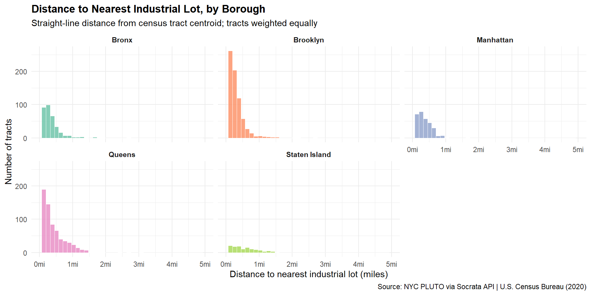
### Distance-Band Analysis
The binary gap classification (covered vs. not) masks variation in how far
residents actually are from industrial land. This section reports the share
of population within each distance band, by borough, and the median straight-line
distance from tract centroid to the nearest industrial lot.
Two distance measures are in use here and they give different numbers
intentionally. The borough table (below) classifies a tract as "covered" if
any part of it intersects a 1-mile buffer -- the most generous possible
reading. The distance table here uses the tract centroid, which is stricter:
a large tract whose center sits 1.1 miles away counts as a gap by centroid
even if its edge is technically within range. The 0.7% city-wide figure
comes from the buffer method; the centroid method shows about 6% of Queens
residents and 12% of Staten Island residents more than a mile from industrial
land.
```{r}
#| label: distance-bands
# Requires dist_to_nearest_miles column added by 02_spatial_analysis.R
bands <- c(0.5, 1, 2, 3)

tracts_with_borough <- nyc_tracts |>
  st_drop_geometry() |>
  mutate(
    borough = case_when(
      substr(GEOID, 3, 5) == "061" ~ "Manhattan",
      substr(GEOID, 3, 5) == "047" ~ "Brooklyn",
      substr(GEOID, 3, 5) == "081" ~ "Queens",
      substr(GEOID, 3, 5) == "005" ~ "Bronx",
      substr(GEOID, 3, 5) == "085" ~ "Staten Island",
      TRUE ~ NA_character_
    )
  ) |>
  filter(!is.na(population), !is.na(dist_to_nearest_miles), !is.na(borough))

borough_bands <- tracts_with_borough |>
  group_by(borough) |>
  summarise(
    within_0.5mi   = percent(sum(population[dist_to_nearest_miles <= 0.5]) / sum(population), accuracy = 0.1),
    within_1mi     = percent(sum(population[dist_to_nearest_miles <= 1.0]) / sum(population), accuracy = 0.1),
    within_2mi     = percent(sum(population[dist_to_nearest_miles <= 2.0]) / sum(population), accuracy = 0.1),
    within_3mi     = percent(sum(population[dist_to_nearest_miles <= 3.0]) / sum(population), accuracy = 0.1),
    median_dist_mi = round(median(dist_to_nearest_miles, na.rm = TRUE), 2),
    .groups = "drop"
  ) |>
  arrange(desc(median_dist_mi))

# City-wide row
citywide_band <- tracts_with_borough |>
  summarise(
    borough        = "NYC (all)",
    within_0.5mi   = percent(sum(population[dist_to_nearest_miles <= 0.5]) / sum(population), accuracy = 0.1),
    within_1mi     = percent(sum(population[dist_to_nearest_miles <= 1.0]) / sum(population), accuracy = 0.1),
    within_2mi     = percent(sum(population[dist_to_nearest_miles <= 2.0]) / sum(population), accuracy = 0.1),
    within_3mi     = percent(sum(population[dist_to_nearest_miles <= 3.0]) / sum(population), accuracy = 0.1),
    median_dist_mi = round(median(dist_to_nearest_miles, na.rm = TRUE), 2)
  )

band_table <- bind_rows(borough_bands, citywide_band)

kable(
  band_table |>
    select(
      Borough                    = borough,
      `Within 0.5mi`             = within_0.5mi,
      `Within 1mi`               = within_1mi,
      `Within 2mi`               = within_2mi,
      `Within 3mi`               = within_3mi,
      `Median tract dist. (mi)`  = median_dist_mi
    ),
  caption = "Population share within each distance band, by borough (straight-line distance from tract centroid to nearest industrial lot)"
)
```
```{r}
#| label: distance-chart
#| fig-cap: "Distribution of tract-level distances to nearest industrial lot, by borough"
#| fig-height: 5
nyc_tracts |>
  st_drop_geometry() |>
  mutate(
    borough = case_when(
      substr(GEOID, 3, 5) == "061" ~ "Manhattan",
      substr(GEOID, 3, 5) == "047" ~ "Brooklyn",
      substr(GEOID, 3, 5) == "081" ~ "Queens",
      substr(GEOID, 3, 5) == "005" ~ "Bronx",
      substr(GEOID, 3, 5) == "085" ~ "Staten Island",
      TRUE ~ NA_character_
    )
  ) |>
  filter(!is.na(dist_to_nearest_miles), !is.na(borough)) |>
  ggplot(aes(x = dist_to_nearest_miles, fill = borough)) +
  geom_histogram(bins = 40, alpha = 0.8, color = "white", linewidth = 0.2) +
  facet_wrap(~borough, nrow = 2) +
  scale_x_continuous(limits = c(0, 5), labels = function(x) paste0(x, "mi")) +
  scale_fill_brewer(palette = "Set2", guide = "none") +
  labs(
    title    = "Distance to Nearest Industrial Lot, by Borough",
    subtitle = "Straight-line distance from census tract centroid; tracts weighted equally",
    x        = "Distance to nearest industrial lot (miles)",
    y        = "Number of tracts",
    caption  = "Source: NYC PLUTO via Socrata API | U.S. Census Bureau (2020)"
  ) +
  theme_minimal() +
  theme(
    plot.title         = element_text(face = "bold"),
    strip.text         = element_text(face = "bold")
  )
```
### Borough Breakdown
```{r}
#| label: borough-table
borough_table <- borough_summary |>
  select(borough, coverage, tracts, population) |>
  filter(!is.na(borough)) |>
  tidyr::pivot_wider(
    names_from  = coverage,
    values_from = c(tracts, population),
    values_fill = 0
  ) |>
  mutate(
    `% in Gap` = scales::percent(
      population_Underserved / (population_Served + population_Underserved),
      accuracy = 0.1
    )
  ) |>
  arrange(desc(population_Underserved / (population_Served + population_Underserved))) |>
  select(
    Borough          = borough,
    `Gap Tracts`     = tracts_Underserved,
    `Covered Tracts` = tracts_Served,
    `Pop. in Gap`    = population_Underserved,
    `% in Gap`
  )

kable(
  borough_table,
  format.args = list(big.mark = ","),
  caption     = "Industrial land proximity by borough (tract covered if any part lies within 1 mile of an industrial lot)"
)
```
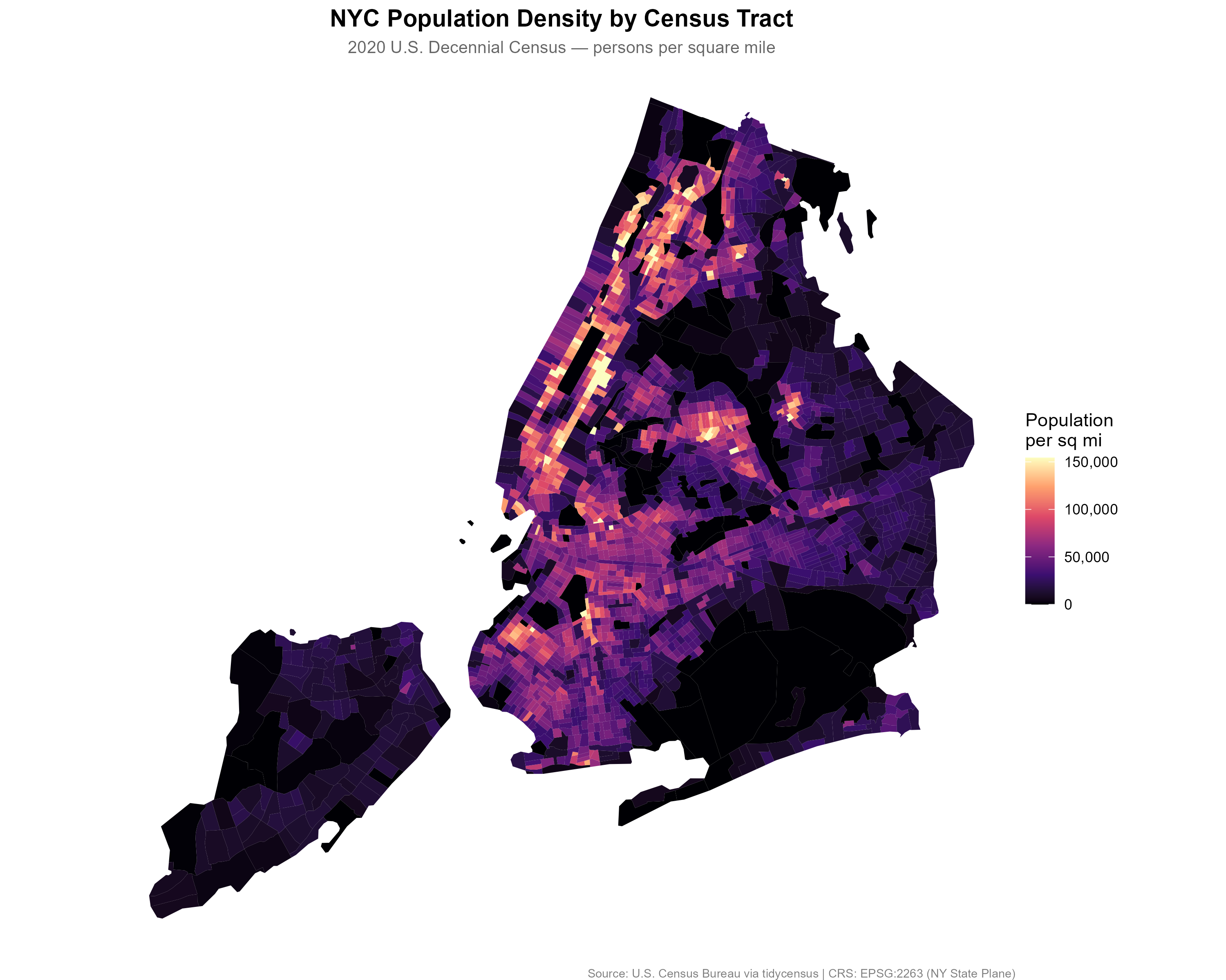
### Map 1: Population Density
The population density map establishes the baseline: where are people
concentrated across the five boroughs? Manhattan's core shows the highest
densities, exceeding 150,000 persons per square mile in some tracts. The
outer boroughs show more moderate densities with significant variation
between neighborhoods.
```{r}
#| label: map1
#| fig-cap: "NYC population density by census tract, 2020 Decennial Census"
knitr::include_graphics(here("output/maps/map1_population_density.png"))
```
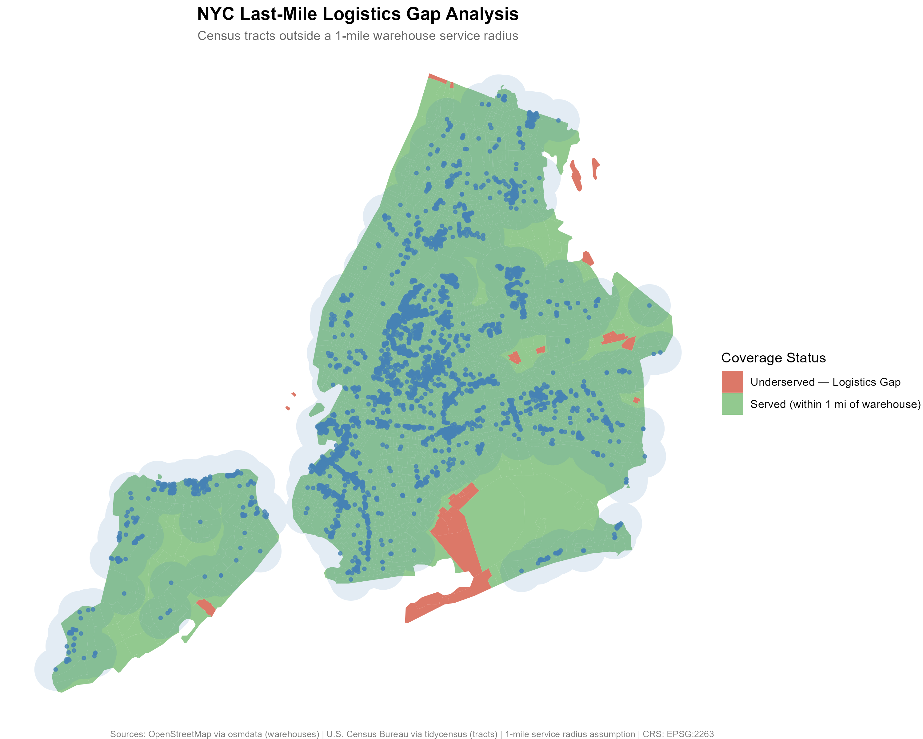
### Map 2: Industrial Land Proximity Gap
The gap map overlays three layers of information: census tract proximity
status (green = within 1 mile of an industrial lot, red = outside 1 mile),
the merged 1-mile coverage zone (light blue halo), and individual
industrial lot locations (blue points).
```{r}
#| label: map2
#| fig-cap: "NYC industrial land proximity gaps — census tracts outside a 1-mile radius of any industrial lot"
knitr::include_graphics(here("output/maps/map2_logistics_gaps.png"))
```
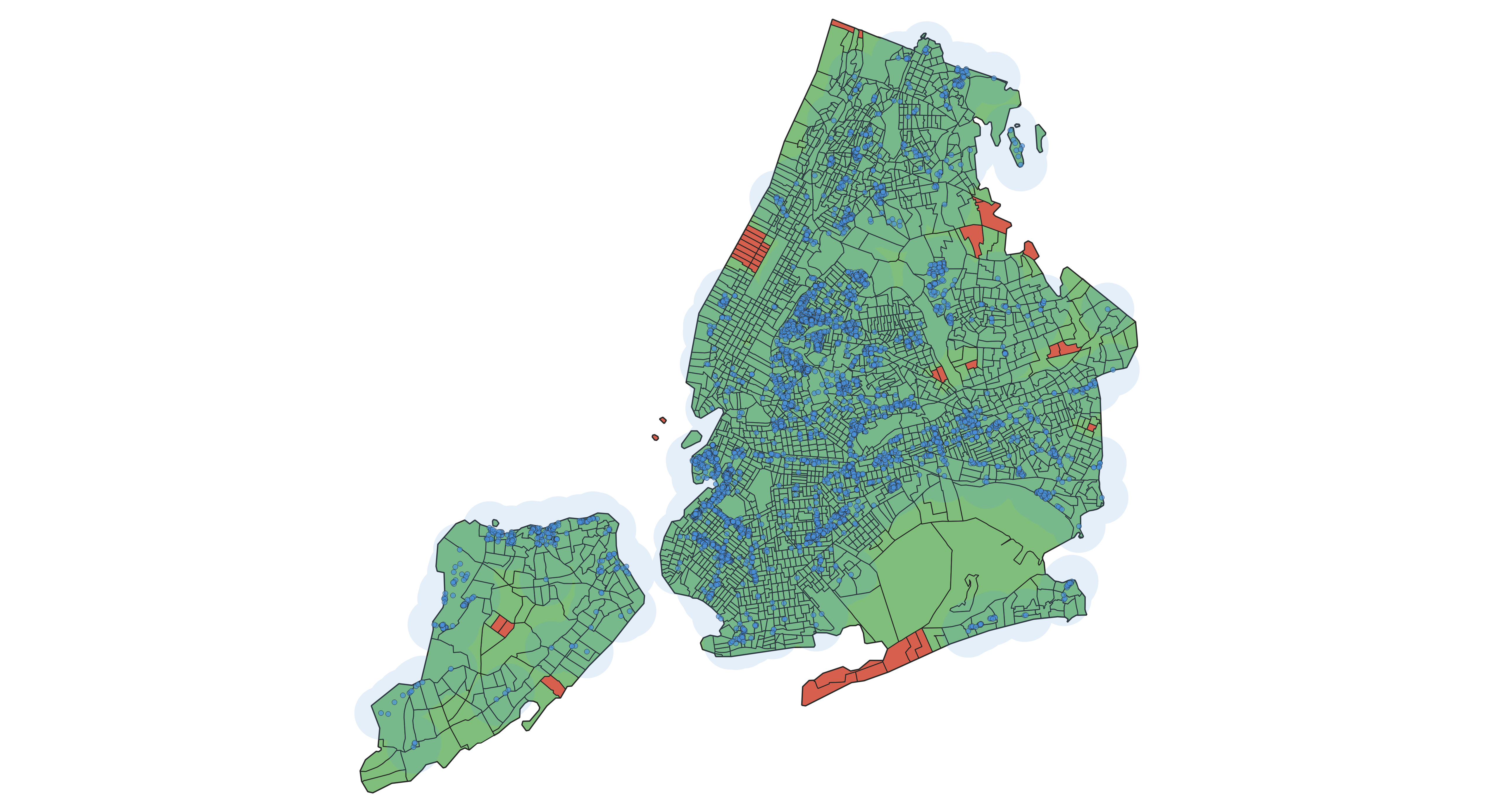
### Map 3: QGIS Cartographic Export
The following map was produced directly in QGIS 3.44 LTR using the same
analysis layers exported from R. It demonstrates the full geospatial workflow
— data processed in R, layers loaded and styled in QGIS, and exported as a
cartographic output.
```{r}
#| label: map3
#| fig-cap: "QGIS styled map export — borough boundaries, census tract proximity status, 1-mile industrial land buffer, and industrial lot locations"
knitr::include_graphics(here("output/maps/qgis_map_export.png"))
```
### Borough-Level Bar Chart
```{r}
#| label: bar-chart
#| fig-cap: "Population outside 1-mile industrial radius, by borough"
#| fig-height: 5
underserved_by_borough <- borough_summary |>
  filter(coverage == "Underserved", !is.na(borough)) |>
  arrange(desc(population))

ggplot(underserved_by_borough,
       aes(x = reorder(borough, population), y = population)) +
  geom_col(fill = "#d6604d", alpha = 0.85) +
  geom_text(
    aes(label = comma(population)),
    hjust  = -0.1,
    size   = 3.5,
    color  = "gray30"
  ) +
  coord_flip() +
  scale_y_continuous(
    labels = comma,
    expand = expansion(mult = c(0, 0.15))
  ) +
  labs(
    title    = "Residents Outside 1-Mile Industrial Land Radius, by Borough",
    subtitle = "Census tracts with no industrial lot (PLUTO code 06) within 1 mile",
    x        = NULL,
    y        = "Population",
    caption  = "Source: U.S. Census Bureau (2020) | NYC PLUTO via Socrata API"
  ) +
  theme_minimal() +
  theme(
    plot.title         = element_text(face = "bold"),
    panel.grid.major.y = element_blank()
  )
```
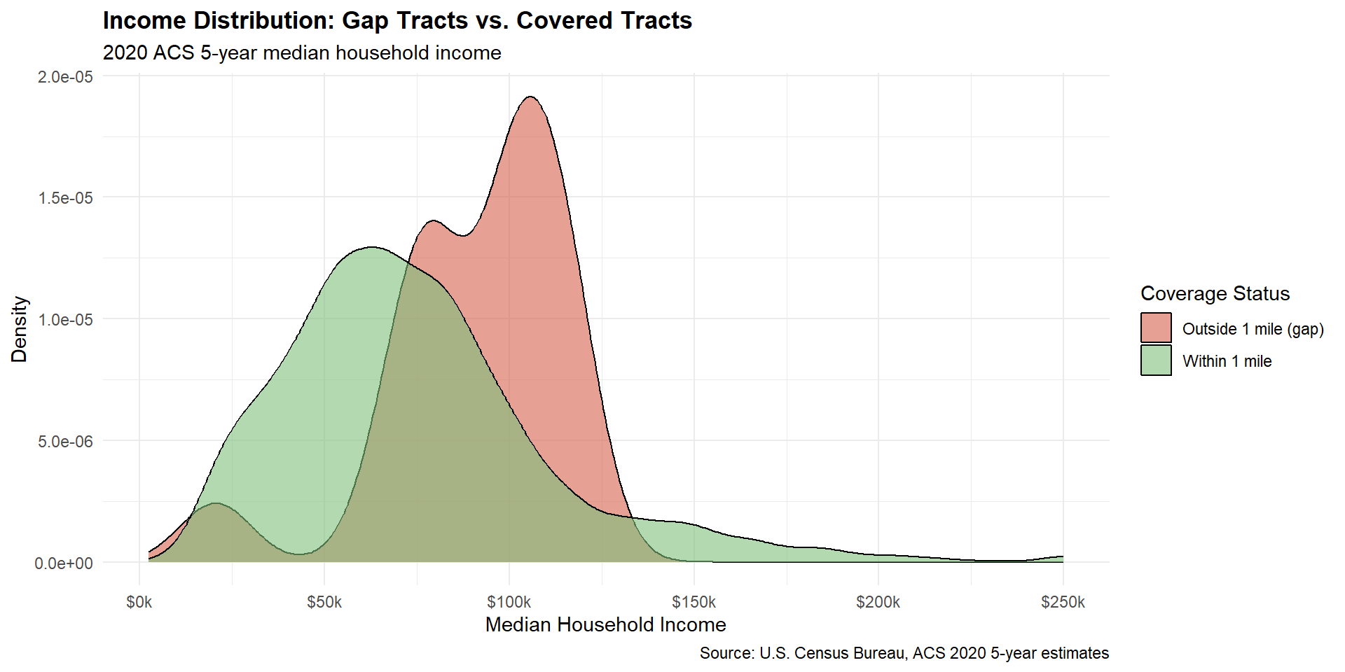
### Income Analysis: Does Wealth Drive the Pattern?
The gap tracts are concentrated in outer Queens and Brooklyn. That raises an
obvious question: are these areas systematically wealthier, and if so, does
income explain why industrial land is absent -- through zoning exclusion, land
costs, or political influence? To examine this, I pull 2020 ACS median
household income by tract and compare distributions across distance bands.
```{r}
#| label: income-pull
# Load pre-pulled income data (pulled in 01_data_pull.R)
# Avoids calling the Census API at render time.
income_data <- readRDS(here("data/processed/nyc_income.rds"))

nyc_tracts_income <- nyc_tracts |>
  st_drop_geometry() |>
  left_join(income_data, by = "GEOID") |>
  filter(!is.na(median_income))
```
```{r}
#| label: income-by-band
band_table <- nyc_tracts_income |>
  mutate(band = cut(
    dist_to_nearest_miles,
    breaks = c(0, 0.25, 0.5, 1, Inf),
    labels = c("0-0.25 mi", "0.25-0.5 mi", "0.5-1 mi", ">1 mi"),
    include.lowest = TRUE
  )) |>
  group_by(band) |>
  summarise(
    tracts        = n(),
    residents     = sum(population, na.rm = TRUE),
    median_income = median(median_income, na.rm = TRUE),
    .groups = "drop"
  )

kable(
  band_table,
  col.names   = c("Distance Band", "Tracts", "Residents", "Median Household Income"),
  format.args = list(big.mark = ","),
  digits      = 0,
  caption     = "Median household income by distance to nearest industrial lot (2020 ACS 5-year)"
)
```
```{r}
#| label: income-wilcox
wt <- wilcox.test(
  median_income ~ I(dist_to_nearest_miles > 0.5),
  data = nyc_tracts_income
)
```
```{r}
#| label: income-summary
income_summary <- nyc_tracts_income |>
  group_by(served) |>
  summarise(
    tracts        = n(),
    median_income = median(median_income, na.rm = TRUE),
    .groups = "drop"
  ) |>
  mutate(group = ifelse(served, "Within 1 mile of industrial land", "Outside 1 mile (gap)"))

kable(
  income_summary |> select(group, tracts, median_income),
  col.names   = c("Group", "Tracts", "Median Household Income"),
  format.args = list(big.mark = ","),
  caption     = "Median household income: gap tracts vs. covered tracts (2020 ACS 5-year)"
)
```
```{r}
#| label: income-chart
#| fig-cap: "Median household income distribution: gap tracts vs. covered tracts"
#| fig-height: 5
ggplot(nyc_tracts_income, aes(x = median_income, fill = served)) +
  geom_density(alpha = 0.6) +
  scale_fill_manual(
    values = c("FALSE" = "#d6604d", "TRUE" = "#7fbf7b"),
    labels = c("FALSE" = "Outside 1 mile (gap)", "TRUE" = "Within 1 mile")
  ) +
  scale_x_continuous(labels = dollar_format(scale = 1/1000, suffix = "k")) +
  labs(
    title    = "Income Distribution: Gap Tracts vs. Covered Tracts",
    subtitle = "2020 ACS 5-year median household income",
    x        = "Median Household Income",
    y        = "Density",
    fill     = "Coverage Status",
    caption  = "Source: U.S. Census Bureau, ACS 2020 5-year estimates"
  ) +
  theme_minimal() +
  theme(plot.title = element_text(face = "bold"))
```
```{r}
#| label: income-interpretation
all_gap_median <- median(
  nyc_tracts_income$median_income[!nyc_tracts_income$served], na.rm = TRUE
)
served_median <- median(
  nyc_tracts_income$median_income[nyc_tracts_income$served], na.rm = TRUE
)

cat(
  "Median income, gap tracts (all NYC):  $", comma(round(all_gap_median)), "\n",
  "Median income, covered tracts:        $", comma(round(served_median)), "\n",
  "Gap tracts with income data:          ",
  sum(!nyc_tracts_income$served), "of", sum(!nyc_tracts$served), "\n"
)
```
Median household income rises monotonically with distance from industrial land
across all four distance bands: $63,708 within 0.25 miles, $66,704 at 0.25--0.5
miles, $84,558 at 0.5--1 mile, and $90,379 beyond 1 mile. The largest step is
between the 0.25--0.5 mile band ($66,704) and the 0.5--1 mile band ($84,558),
a gap of roughly $18,000. A Wilcoxon rank-sum test comparing tracts within
0.5 miles to tracts beyond 0.5 miles confirms the difference is not noise
(p < 0.001, across 2,206 tracts with income data).
The binary gap comparison (the 31 gap tracts vs. the rest) tells the same
story: gap tracts median $`r comma(round(all_gap_median))` vs. covered tracts
$`r comma(round(served_median))`. But the distance-band table is more informative
because it shows the gradient holds continuously, not just at the 1-mile cutoff.
The data cannot distinguish between two explanations: affluent neighborhoods may
have successfully excluded industrial uses through zoning, or those neighborhoods
may simply sit at the outer edges of where the city's industrial corridors
historically developed. Separating geography from politics would require zoning
history and land use change data over time. What the data does establish is that
the income gradient is real, city-wide, and statistically robust.
---
## Discussion
### Key Findings
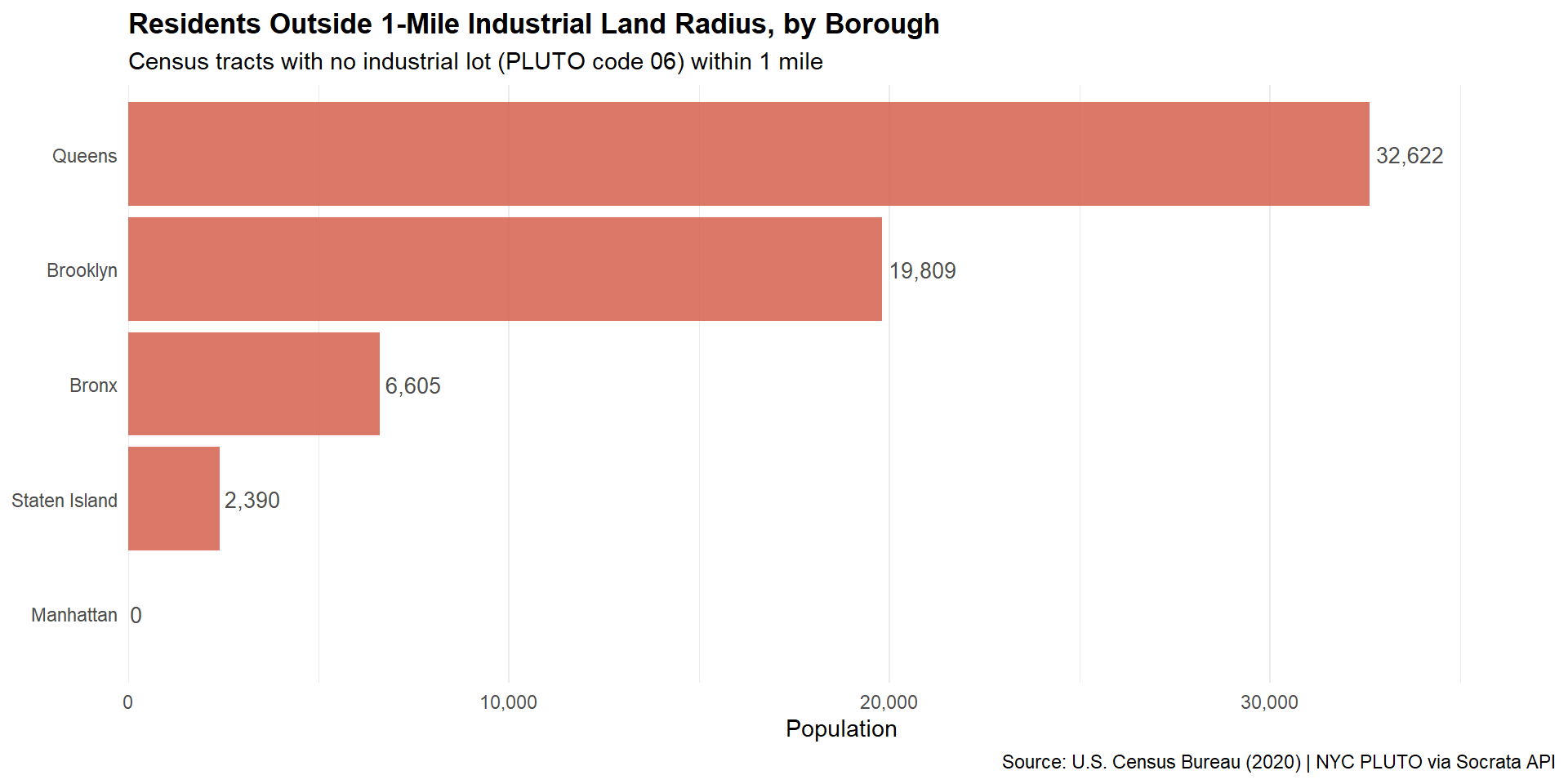
Queens has the largest gap population (32,622 residents across 13 tracts),
followed by Brooklyn (19,809 across 11 tracts). Both sets of gap tracts sit at
the outer edges of their boroughs, distant from the industrial corridors
concentrated along the waterfront and freight routes closer to the urban core.
Manhattan has only one gap tract (GEOID 36061000100, Census Tract 1), with
zero counted residents. Its centroid falls at approximately 40.695°N, 74.043°W,
in the harbor southwest of the Battery -- consistent with harbor islands
(Governors Island, Ellis Island, or Liberty Island) that carry no permanent
residents. Zero is most likely a true count, not a differential privacy
artifact. Manhattan's near-complete industrial land coverage otherwise reflects
the density of lots in specific corridors (West Side railyards, Meatpacking
District, Hudson Yards area).
Median household income rises monotonically with distance from industrial land
across all four distance bands, from $63,708 within a quarter mile to $90,379
beyond a mile. The largest step is between the 0.25--0.5 mile band ($66,704)
and the 0.5--1 mile band ($84,558). A Wilcoxon rank-sum test comparing tracts
within 0.5 miles to tracts beyond 0.5 miles confirms the gradient is
statistically significant (p < 0.001, across 2,206 tracts). The data cannot
say whether this reflects deliberate zoning exclusion or simply the geography
of where industrial corridors developed, but the pattern itself is robust. The
Manhattan gap tract has no income data, since it has no counted population.
The distance-band analysis adds resolution beyond the binary gap classification.
About 16% of New Yorkers (96.6% within a mile minus 80.4% within half a mile)
live in the 0.5--1 mile band. Staten Island stands out with the longest median
tract distance (0.50 miles, vs. 0.21--0.31 for the other four boroughs).
Queens has a shorter median (0.27 miles) but a longer right tail: about 6% of
Queens residents are more than a mile from industrial land by the centroid
measure, the second-highest share after Staten Island.
### Limitations
**Broad land use category.** According to the NYC DCP PLUTO Data Dictionary,
land use code 06 maps to building classes E* (warehouses), F* (factories), and
L* (loft buildings). Factories and lofts are included alongside
distribution-oriented warehouses, and the category gives no indication of
whether a lot hosts an active logistics operation. L* specifically includes
converted loft buildings and self-storage facilities that generate little
noise or truck traffic -- meaningfully different from a large active warehouse.
This analysis measures proximity to industrial land as a class -- it does not
distinguish a 500,000 sq ft fulfillment center from a converted loft building
or an inactive factory floor. Including L* lots weakens the "industrial
facility" proxy and likely understates the income gradient around genuinely
heavy industrial uses. A more operationally precise analysis would require
commercial real estate data (CoStar, CBRE) or cross-referencing with business
license records to isolate active logistics facilities.
**Edge effect.** This analysis counts only NYC-classified lots. Major
distribution hubs in New Jersey and just outside the city line in Nassau and
Westchester are excluded. The effect is largest for Staten Island, which sits
adjacent to major New Jersey logistics corridors in Elizabeth and Linden; its
distance numbers would look materially different if those lots were included.
**The 1-mile threshold.** A tract 1.1 miles from a lot is counted as a gap;
one at 0.9 miles is not. The distance-band table partially addresses this by
reporting continuous bands, but the binary classification in the maps and
borough table still uses the fixed threshold.
**Straight-line distance is not travel time.** Proximity to industrial land
says nothing about road network connectivity, traffic conditions, loading
access, or building entry -- the actual constraints that determine delivery
reach in an urban environment.
### What the Income Gradient Implies for Compensation
The core finding is that NYC census tracts closer to industrial land have
lower median household incomes, and the gradient is continuous and
statistically robust. This does not prove that industrial proximity *causes*
lower incomes -- the causal story runs in at least two directions. Industrial
corridors may have developed where land was already cheap (lower-income areas).
Or affluent neighborhoods may have used zoning to exclude industrial uses over
time, making the correlation partly a product of political power. Distinguishing
those explanations requires zoning history data this analysis does not include.
What the gradient does support is a directional reading: across 2,206 NYC
tracts, proximity to industrial land is consistently associated with lower
household income. People with more resources tend to live farther from
industrial land. That pattern is consistent with the Netherlands research
finding a 15% property value discount within 250 meters of industrial sites,
though the two measures capture different things (income sorting vs. asset
value).
**Back to the $10,000 question.** NorthPoint offered Hazle Township residents
$10,000 -- a one-time payment -- to accept a 1,300-acre data center. The
Netherlands study gives the clearest empirical benchmark: homes within 250
meters of industrial sites sold for roughly 15% less. If a home near the
facility is worth $200,000, that is a $30,000 loss in asset value -- three
times the NorthPoint offer. The discount fades with distance; by roughly 1.4
miles it is near zero, so homes closest to the facility bear the largest loss.
A flat $10,000 to everyone regardless of distance ignores that geography
entirely.
The NYC income gradient points the same direction. Tracts within 0.25 miles
of industrial land have a median income of $63,708; tracts beyond 1 mile reach
$90,379. That $26,671 gap reflects sorting rather than a direct cost to any
individual household, and should not be read as an annual figure. But it
reinforces the Dutch finding: proximity to industrial land is something people
with options choose to avoid.
None of this means developers should not build. It means the compensation
question deserves an empirical basis rather than an arbitrary one. Relevant
inputs would include: the distance from the facility to each household, local
property values before and after comparable facilities opened nearby, the
expected duration of impacts (noise, traffic, visual), and whether payments
should be structured as one-time checks or ongoing annual compensation tied
to the facility's operating life.
### Implications for the AI Data Center Debate
The current conflict over data center siting is partly a zoning fight, partly
an AI anxiety fight, and partly a legitimate dispute over who pays for
infrastructure that benefits a much larger population. In Q2 2026 alone,
community resistance stalled $68 billion in data center projects across the U.S.
[TechCrunch](https://techcrunch.com/2026/09/22/everyone-can-find-a-reason-to-dislike-data-center-construction/)
reported in September 2026 that "everyone can find a reason to dislike data
center construction" -- from noise and water use to AI ethics to simple
neighborhood character concerns.
The [Brookings Institution](https://www.brookings.edu/articles/data-center-backlash-signals-a-fight-over-ai-power/)
framed it as a democratic accountability problem: if AI infrastructure is
built wherever companies choose, with local governments as the only check,
communities end up negotiating individually against well-resourced developers
without any common framework for what fair compensation looks like.
NYC's industrial land income gradient does not resolve that, but it offers
one empirical anchor. Across 2,206 tracts, income rises consistently with
distance from industrial land. That sorting pattern, combined with the Dutch
property value evidence, suggests the question of what residents are owed is
empirical, not just political -- and that a flat $10,000 is not derived from
any such calculation.
Whether the comparison between NYC's industrial lots and a Pennsylvania data
center is close enough to matter is a judgment call. The land uses are
different. The geography is different. But the core mechanism -- a large
industrial facility arrives near a residential area, generating noise, traffic,
and visual impact -- is similar enough that the income gradient finding is at
minimum a reasonable order-of-magnitude reference, and significantly better
than no empirical basis at all.
---
## Reproducibility
All data is pulled from public APIs at runtime. To reproduce this analysis
from scratch:
```r
# 1. Install packages and create folder structure
source("setup.R")

# 2. Pull all data from APIs
source("analysis/01_data_pull.R")

# 3. Run spatial analysis (computes covered/gap status and dist_to_nearest_miles)
source("analysis/02_spatial_analysis.R")

# 4. Export maps
source("analysis/03_maps.R")

# 5. Render this report
quarto::quarto_render("report/index.qmd")
```
**R version:** `r R.version$version.string`
**Key packages:** tidycensus `r packageVersion("tidycensus")`,
sf `r packageVersion("sf")`,
ggplot2 `r packageVersion("ggplot2")`
---
## Data Citations
U.S. Census Bureau. (2020). *2020 Decennial Census Redistricting Data
(Public Law 94-171) Summary File*. Retrieved via the tidycensus R package.
U.S. Census Bureau. (2020). *American Community Survey 5-Year Estimates:
Median Household Income (B19013)*. Retrieved via the tidycensus R package.
NYC Department of City Planning. (2024). *PLUTO: Primary Land Use Tax Lot
Output*. NYC Open Data. https://data.cityofnewyork.us/resource/64uk-42ks.json
U.S. Census Bureau. (2024). *TIGER/Line Shapefiles: Counties*. Retrieved
via the tigris R package.
---
## References and Further Reading
de Vor, F., & de Groot, H. L. F. (2011). *The Impact of Industrial Sites on
Residential Property Values: A Hedonic Pricing Analysis from the Netherlands.*
Regional Studies, 45(5), 609--623. Key finding: 15% price discount within 250
meters of industrial sites, fading to near zero at 2,250 meters (roughly 1.4
miles). Based on 70,684 home sales.
https://papers.tinbergen.nl/09035.pdf
Data Center Watch / Parameter.io. (2026). *Community Resistance Stalls $68
Billion Worth of AI Data Center Developments.*
https://parameter.io/community-resistance-stalls-68-billion-worth-of-ai-data-center-developments/
Wheeler, T. (2026). *Data Center Backlash Signals a Fight Over AI Power.*
Brookings Institution.
https://www.brookings.edu/articles/data-center-backlash-signals-a-fight-over-ai-power/
Alcorn, C. (2026). *Data center developer offers $10,000 checks to 4,500
households if 1,300-acre facility is approved.* Tom's Hardware.
https://www.tomshardware.com/tech-industry/data-centers/data-center-developer-offers-usd10-000-checks-to-4-500-households-if-the-1-300-acre-facility-is-approved-locals-push-back-over-noise-and-bribe-concerns
George Mason University, Schar School of Policy and Government. (2025).
*Study: Home Prices Are Higher When the House Is Near a Data Center.*
https://schar.gmu.edu/news/2025-11/study-home-prices-are-higher-when-house-near-data-center
Coldewey, D. (2026, September 22). *Everyone can find a reason to dislike
data center construction.* TechCrunch.
https://techcrunch.com/2026/09/22/everyone-can-find-a-reason-to-dislike-data-center-construction/
Haber, M. (2026). *How Data Centers Are Set to Impact the Value of Your Home.*
Newsweek.
https://www.newsweek.com/how-data-centers-are-set-to-impact-the-value-of-your-home-11939599
---
## AI Usage Disclosure
This project was developed with assistance from Claude (Anthropic) as a
collaborative coding and methodology tool. Claude helped structure the R
scripts, debug API connectivity issues during data acquisition, and draft
the prose in this report. All analytical decisions — including the choice
of 1-mile service radius, the PLUTO land use classification, and the
interpretation of results — were made and reviewed by the author. All code
was tested and executed locally by the author prior to publication.